
Submitted:
06 December 2023
Posted:
15 December 2023
You are already at the latest version
Abstract
In our latest studies with the help of the self-similar Ansatz we derived new type of 1
solutions for the regular diffusion equation which are much more complex than the well-known 2
Gaussian and error functions. These solutions contain additional Kummer’s M and Kummer’s U 3
functions with quadratic argument. In the present treaties we perform an analogous analysis for the 4
regular diffusion equation which has a complex diffusion coefficient. Formally, it is equivalent to 5
the free Schrödinger equation however it is far from being trivial how the solutions can be given 6
quantum mechanical interpretation. We investigate both the one dimensional Cartesian and the 7
spherical symmetric equations. We find solutions which fulfill the L2 integrability criteria therefore 8
might have quantum mechanical relevance in the future.
Keywords:
schrödinger equation
; complex diffusion
; self-similar Ansatz
1. Introduction
It is an evidence that diffusion (or heat conduction) is a fundamental physical process which attracted enormous intellectual interest from mathematician, physicists and engineers in the last two centuries. The existing literature about diffusion (or again about heat conduction) is immense, therefore we just mention some basic textbooks [1,2,3,4].
When the diffusion coefficient became complex we arrive to the free Schrödinger equation which is one of the corner stones of non-relativistic quantum mechanics. The achieved knowledge about the Schrödinger equation can also fill libraries. Some basic well-known text book are the following [5,6,7,8]. The similarities and differences with ordinary diffusion can be studied in books like [9] or [10].
Two decades ago one of us (I.F. Barna) also worked with the usual quantum mechanics as a regular tool to investigate photoionization of He atoms [11].
In our study to derive analytic results we will apply the reduction mechanism which is a powerful tool to analyze linear and non-linear partial differential equations (PDE) or PDE systems transforming them to linear (or non-linear) ordinary differential equations (ODEs) or ODE systems. In numerous cases these equations can be solved with analytical means. The obtained solutions give a glimpse into the general and global properties of the original PDE equation e.g. gives us the asymptotic power-law properties, discontinuities, oscillations etc. Under the reduction mechanism we mean, that coupling the original temporal ’t’ and the spatial variable ’x’ (or ’r’) to a new type of variable and therefore transforming the original PDE to an ODE depending on the variable of . It is evident that numerous kind of reduced variable can be considered and constructed. In the present case we are going to use the physically most relevant self-similar Ansatz.
In our former studies in a research paper [12] and in a book chapter [13] we applied the self-similar Ansatz to the Madelung equation which is a fluid mechanical analogue of the Schrödinger equation. We derived that the fluid density is proportional to the square of the Bessel function with a quadratic argument. Therefore the density function had countable infinite zeros which is a remarkable and less usual property in fluid mechanics and originated from quantum mechanics.
The present study organically follows our former analysis in which we in-depth investigated the regular diffusion equation [14,15,16]. Now we extend our research to the complex diffusion processes which is formally equivalent to the free Schrödinger equation. We address both the one dimensional Cartesian and the spherically symmetric equations as well. After the mathematical analysis of the solutions we try to give a quantum mechanical interpretation of our results. We investigate the parameter dependencies of the results and find a regime where the integrability is fulfilled.
The study ends with a short summary and an outlook which shows the direction of possible future investigations.
2. Theory and Results
2.1. Overview of the solutions for the real diffusion
Before we derive the generalized self-similar solutions for the Schrödinger equation we briefly summarize our former results which were obtained for regular diffusion considering the Cartesian and the spherical symmetric cases as well.
2.1.1. Cartesian case
Having in mind that the general diffusion process is three dimensional we consider only one Cartesian coordinate, therefore the equation reads
where is the distribution of the particle concentration in space and time and from physical reasons D is the diffusion coefficient which is a positive real constant. in the equation above is considered up to a constant, consequently it may also refer to the concentration above or around the average. The function fulfills the necessary smoothness conditions with existing continuous first and second derivatives. Numerous physics textbooks gives us the derivation how the fundamental (the Gaussian) solutions can be obtained e.g. [1,2]. In the well-known work of Bluman and Cole in 1969 [17] numerous analytic solutions were given for the diffusion equation, and they arrived to a certain level.
In our analysis we apply the self-similar Ansatz in the form of
where and are the self-similar exponents being real numbers describing the decay and the spreading of the solution in time and space. These properties makes this Ansatz physically extraordinary relevant and was first introduced by Sedov [18]. For the present diffusion equation, after some trivial algebra we get:
and there is a clear-cut time-independent ordinary differential equation (ODE) of
With the choice of and setting the first integration constant to zero we get back the well-known Gaussian solution.
This is the so-called fundamental solution and sometimes referred to as solution – by mathematicians – because for the . As far as we know this is the simplest and shortest derivation to obtain the fundamental solution from the original PDE of Eq. (1). Therefore this Ansatz is original among others and can help to find physically relevant disperse solutions to other physical systems like the Bénard convection problem [19] or a heated boundary layer flow [20].
Using the formula manipulating software package Maple 12 for general real , the solutions read as:
where and are the Kummer’s M and Kummer’s U functions. For more details consult the NIST Handbook [21]. In the following we will analyze this form. For completeness we have to mention that, with another software Mathematica an alternative formulations of the result is possible in the form of
where is the Hermite polynomial (if is a non-negative integer) and is the hypergeometric function. (A key equation between the two formulation is the transformation of [22] 13.6.18.) The first part of the solutions, are the even Hermite polynomials which form a complete orthonormal basis set on the range with the Gaussian weight function for any odd function. (Note, that Hermite polynomials play an extraordinary role in quantum mechanics as the solution of the harmonic oscillator problem [7] which pioneered the way to second quantization or field theory.) At this point for completeness we have to mention that the solutions Eq. (5) according to the value of the parameter, can be divided into four separate groups and each is ordered with essentially different properties:
- the solutions are divergent at large arguments,
- the solution asymptotically becomes a non-zero constant,
- the solutions have a local maxima and a decay to zero at large arguments,
- the solutions have oscillations proportional to the value of and have quicker and quicker decays to zero at larger values.
It is clear to see that most of the resulting functions have odd symmetry, however it can be shown that for some parameters the Kummer’s U functions can have even symmetry [16] as well, which has far reaching consequences. An exhaustive analysis of Eq. (5) was done in our previous studies [14,15,16] which we skip here.
2.1.2. Spherical case
It is a physical evidence that numerous physical systems have spherical symmetry, therefore that kind of diffusion equation is also essential to investigate. The general form of the diffusion equation in cylindrical and spherical coordinate system reads as follows:
where and 2 means Cartesian, cylindrical and spherical symmetry, respectively. Having in mind the valid form of the Ansatz we immediately get the reduced ODE of
with the usual constraints of and . The general solutions read as follows:
The above relation holds for , and Eq. (9) well describes the cylindrical and spherical symmetric solutions. Note that unlike the Cartesian case here all the solutions have even property (symmetrical about the y-axis). With some numerical calculations it can be shown, that the general features of the Cartesian solutions are inherited to the cylindrical and spherical systems as well. So the same type of classification is valid here for different regimes as well.
2.2. Solutions of the complex diffusion equation
2.2.1. The Cartesian case
Continue our analysis with the analogous problem, where the diffusion coefficient becomes complex. In other words let’s investigate the free Schrödinger equation – still in one Cartesian coordinate:
after some trivial modification we arrive to a more suitable form for our analysis:
where is the real "diffusion coefficient" of the equation in the language of diffusion. It is well-known in quantum mechanics, that the free Schrödinger equation has a disperse wave-packet solution which can be written in the form of
exhaustive details of the derivation and the properties can be found in numerous text books like [5,6,8].
Before we derive and discuss our analytic solutions we have to summarize other available results from the literature. We start with the work of Niederer [23] from 1972 who used the maximal kinematical invariance group to solve the free Schödinger equation. Shapalov et al. [24] separated the variables of the stationary Schrödinger equation and presented numerous results. Numerous group theoretical studies were performed from various authors we mention Beckers et al. [25] who investigated in non-relativistic quantum mechanical equations with the subgroups of the Euclidean group, where the Schrödinger or the the Pauli equations were examined with different scalar and vector potentials. It is crucial to emphasize that these studies do not mention our result in the form of Eq. (16). To derive the expression Eq. (12) the method of separation of variables was used, so the temporal ’t’ and the spatial ’x’ variable of the dynamics were handled separately which is the crucial point.
The investigation of wave-packets dynamics is an interesting field in quantum mechanics which helps to visualize the possible wave-particle dualistic dynamics of the quantum particle. As an interesting point we may mention the non-dispersive wave-packet solutions of Berry and Balázs which is based on Airy functions. Such solutions propagates freely without any envelope dispersion, maintaining its shape. [26]. As an extra feature it accelerates undistorted in the absence of an external force field. Nevertheless this properties do not violate Ehrenfest’s theorem. Understanding quantum properties of matter via investigating the wave packed dynamics is a popular method with an immense literature we just mention two reviews [27,28].
The role and the source of time in quantum mechanics is an interesting and open ended question. In the last decades Rost and co workers published different studies about the possible interpretation of time [29,30].
As we learned earlier in the classical diffusion problem one can find the fundamental solution applying self-similar Ansatz, where the time and the temporal variables are not separated (but remained connected) in the self-similar reduced variable . In this sense the classical diffusion process and the free Schrödinger equation ’handles’ space and time dynamical variables in a different way. But to find the key results of this study let’s apply the same self-similar Ansatz as above
to the Eq. (11).
The former physical meaning of and remains the same as was given above. To avoid later mixing we mark with the shape function. After the same trivial algebraic steps we get the same relations for the self-similar exponents:
and a very similar ODE as Eq. (4) in the form of:
With the help of Maple 12 we can easily evaluate the general solution:
where and are still usual real integration constants and and are the Kummer’s M and Kummer’s U functions [21], respectively. (Similarly to the real case an alternative formulation is also available for the solution in the form of:
it is clear to see in this form, that now the even part of solutions are real finite polynomials for negative s. Other properties of that formula is outside the scope of this study.) We concentrate and analyze on the solutions which include the Kummer’s functions. These two equations ( Eq. (5) and Eq. (16) ) are the key results of our analysis.
The essential difference between the solution of the real diffusion equation Eq. (5) and this one Eq. (16) is immediately visible which is the missing Gaussian multiplier function. The second no less negligible difference is the complex argument of both Kummer’s functions.
To perform an in-depth analysis we have to systematically investigate the dependencies of both Kummer’s functions. To accelerate this process it is useful to evaluate the first few Taylor expansion terms of the functions where we can clearly see the role of the parameter.
Try to analyze the properties of this truncated finite series. The first term – Kummer’s M function – is always an odd function and can be defined for arbitrary . Furthermore the odd members are real and the even members are purely complex. For negative half-integer values we get finite polynomials. The second term – the Kummer’s U function – has bit more tricky structure, – due to the analytic properties of the Gamma function [21] - for negative integer s the function has even symmetry, for negative half-integer values (if ) the function has an odd symmetry. For all positive values the function has no even or odd symmetry. The exact parameter dependence of the solution is a complicated problem. To solve this difficulty we apply an empirical method and evaluate the shape functions s for various values. Due to the complex argument of the solution we present the real the complex and the absolute value of the solution. Firstly, figure. (1) shows the results for the Kummer’s M function.
The first, the second and the third figure show the real, the imaginary and the absolute value of function for . Having in mind the Kummer’s transformation formula [21] (13.2.39)
we can find interesting unexpected identities during the analysis like: , or even ,
for the Kummer’s M functions only. This is the reason why only five curves are visible on fig. (1c). Some other curves coincide. A more detailed analysis showed that only for we get oscillatory but decaying solutions which could have later physical interest.
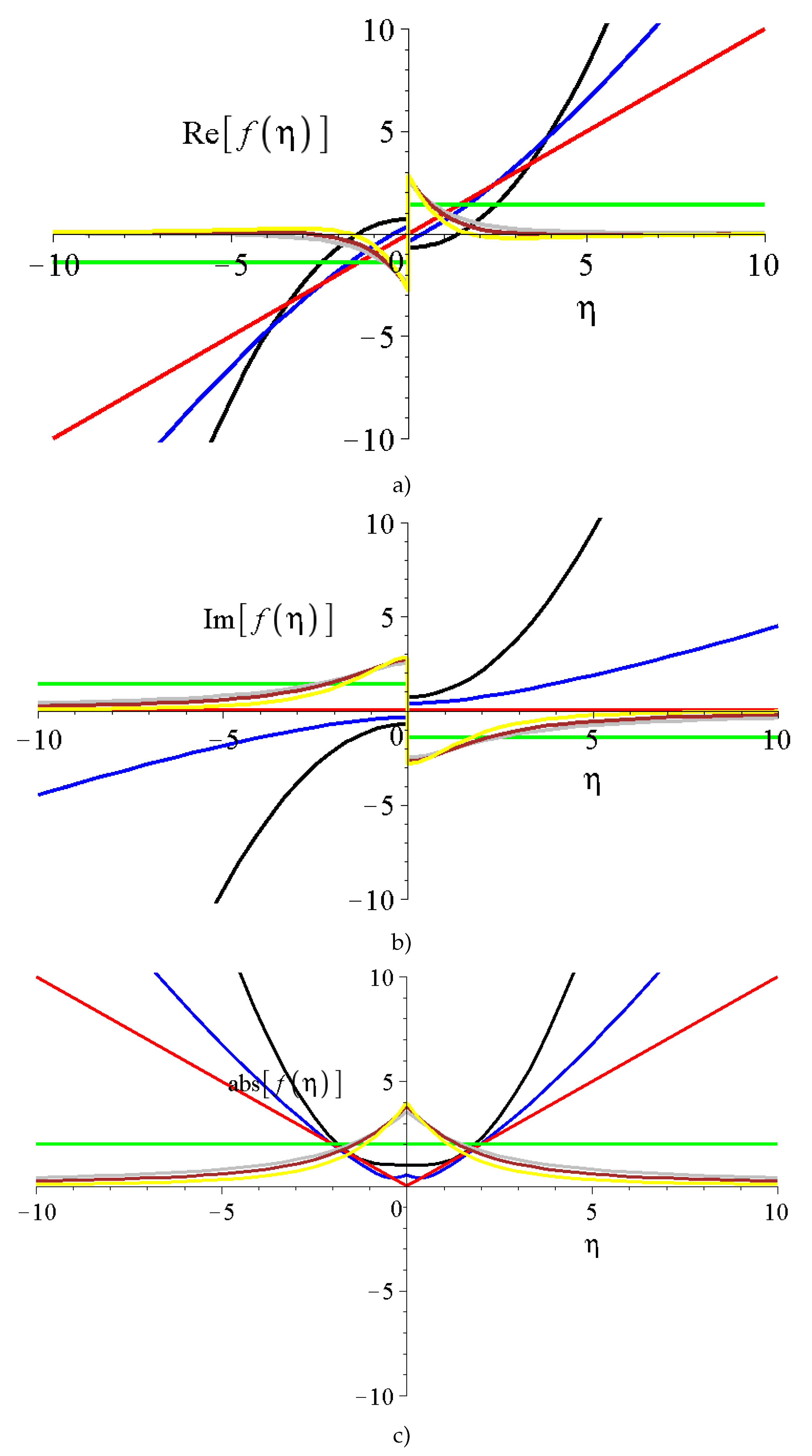
Figure (2) presents the real, imaginary and absolute values of the function for the same values. It is clear to see that, negative values give divergent shape functions which are from physical reasons out of our interest. Positive s give decaying solutions at infinity with an additional cusp in the origin. (Cusp means now a point where the function has a finite numerical value but the derivative is indefinite.)
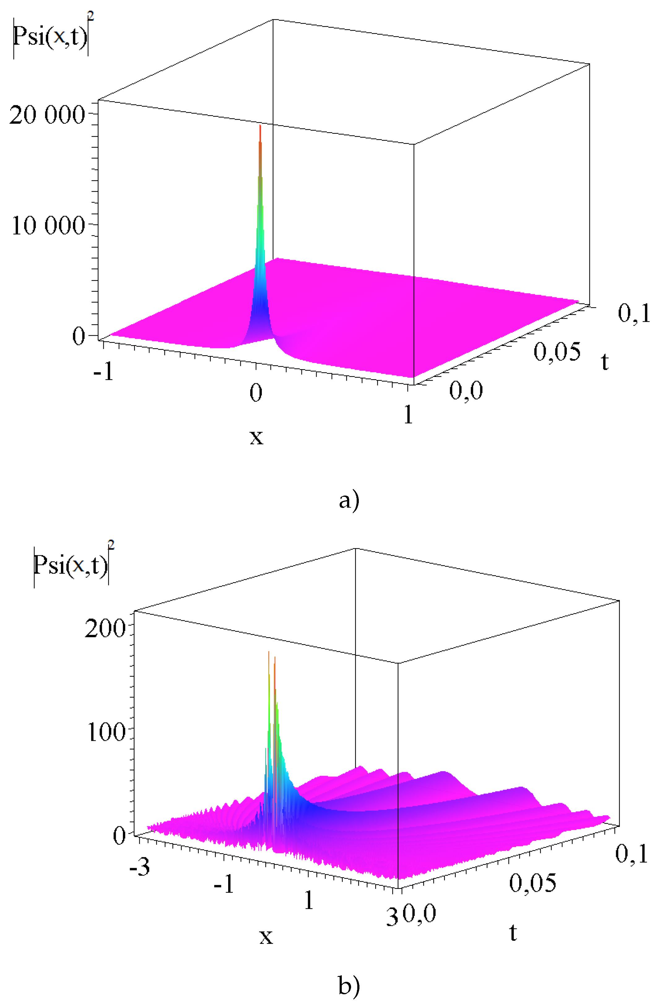
Figure (3) shows the absolute value squared of the wave function for Kummer’s U and Kummer’s M functions if . We found that for all the function has a general temporal and spatial decay. Which is of course not enough for integrability. We performed a large number of numerical integrations to find out the convergence properties and we may say that for the convergence is easy to see with interval doubling. However below the convergence becomes very slow. We have no rigorous mathematical proof where lies the general convergence limit of .
Figure 1.
The and the are the real, the complex and the absolute values of the function in Eq. (16) for . The black,blue,red,green, gray, brown and yellow lines are for and 1, respectively.
Figure 1.
The and the are the real, the complex and the absolute values of the function in Eq. (16) for . The black,blue,red,green, gray, brown and yellow lines are for and 1, respectively.
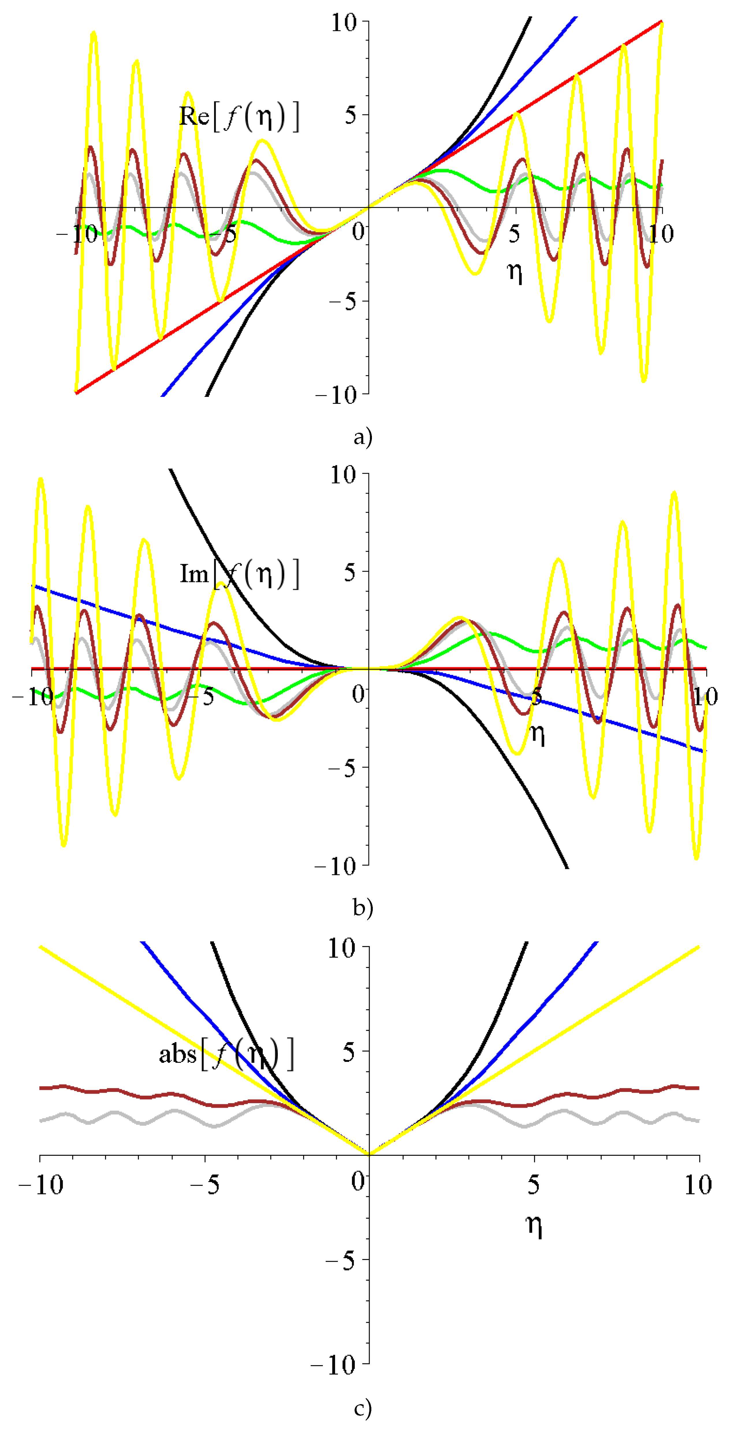
Figure 2.
The and are the real, the complex and the absolute values of the function in for . The black,blue,red,green, gray, brown and yellow lines are for and 1, respectively.
Figure 2.
The and are the real, the complex and the absolute values of the function in for . The black,blue,red,green, gray, brown and yellow lines are for and 1, respectively.
For the other function the situation is a bit more different. For we get the lowest lying oscillating solution which has all local minimums equal to zero. All other solutions lie above this function. Having performed large number of numerical integrations we can say with great certainty no convergence can be achieved for any kind of values.
Figure 3.
The of Eq. (16) for and the upper figure shows the Kummer U and the lower is the Kummer M function, respectively.
Figure 3.
The of Eq. (16) for and the upper figure shows the Kummer U and the lower is the Kummer M function, respectively.
2.2.2. Spherical coordinate system
To have a complete analysis we investigate the spherically case as well:
With the Ansatz of we immediately arrive to a similar ODE of
with the usual constraints of and and diffusion constant of The solutions are:
where and are still the Kummer’s function. Note, the two relevant difference to the Cartesian solutions, are the lack of the extra dependence and the shift in the first argument of the Kummer’s functions. To understand the properties of this solution we have to make a regular parameter study, namely how the solution depends on the free parameter . Figure (4) and figure (5) show the shape functions for different s, for the Kummer’s M and for the Kummer’s U functions. On fig. (4) we clearly see the different kind of properties of the Kummer’s M functions, again the real imaginary and the absolute values are all presented. We can see different regimes again depending on the parameter. Some results are divergent, some solutions have oscillations. Fig. (5) shows the behavior of the Kummer’s U functions. Note, that no oscillations are present here. Of course some solutions are divergent in the origin which is the general property of the Kummer’s U functions.
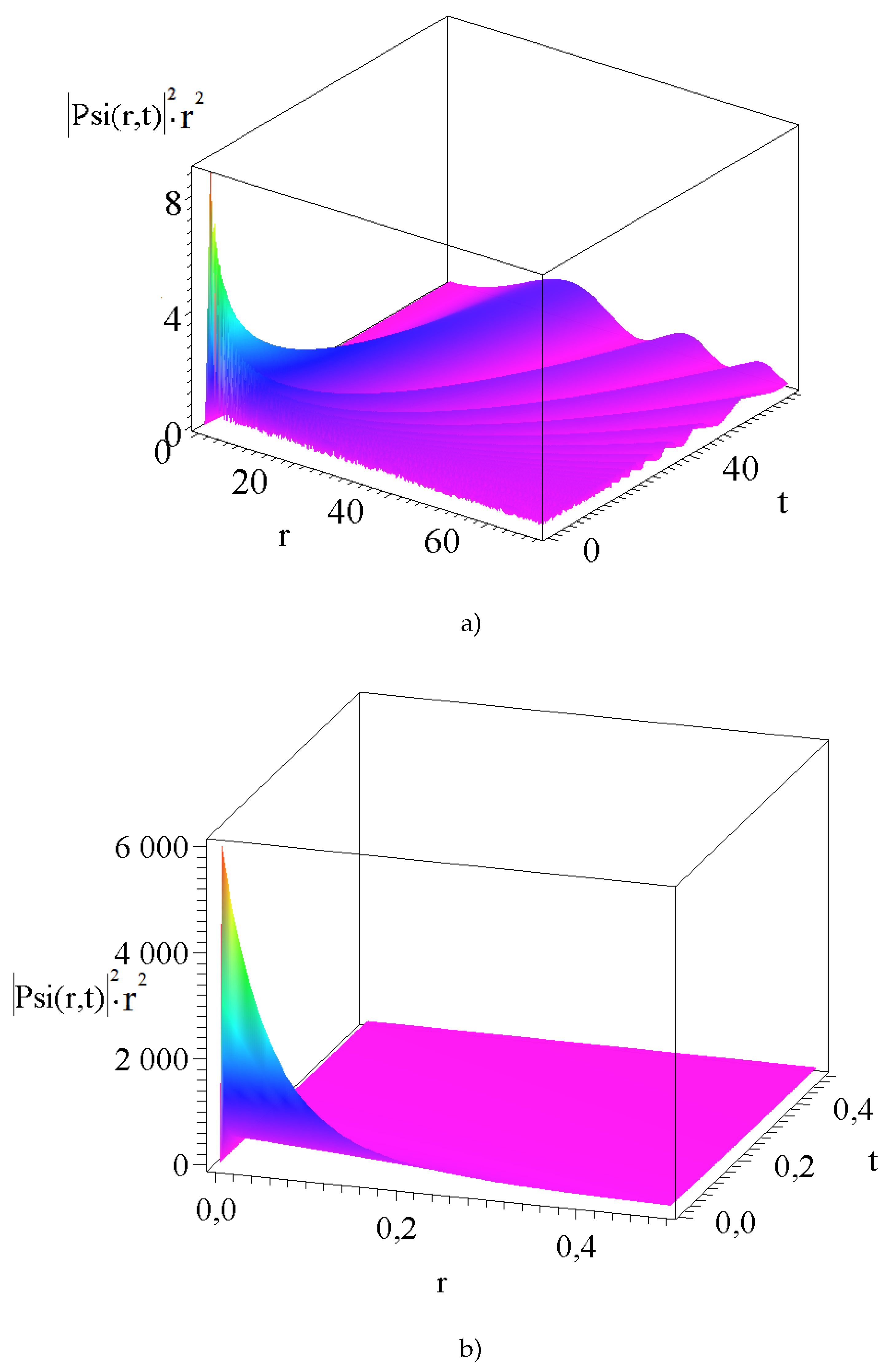
For completeness Fig.(6) presents two possible radial particle density functions expressions. Note, that the Kummer’s M function shows some temporal wavy structure which is familiar from the "ordinary" quantum mechanic solutions. The Kummer’s U functions (which are the irregular solutions) has a very quick decay in space and time with a high value in the origin. Both functions have integrability for some values (e.g. ) therefor these solutions might be considered as "physical wave functions" as well.
3. General consequences
At the end of our study we summarize our results and try to give some interpretation of the obtained results. The first statement is the following due to the linearity of the complex diffusion equation (or the Schrödinger equation) our solutions in principle can be freely added to other physically relevant solutions like the well-known wave packets. However, due to the non-orthogonality of our solutions to the well-known wave packets the integral or norm of such wave function can be evaluated as well. Of course that modifies the initial and boundary conditions and the physical meaning of such a solution will be an important question. It is worth to mention that for same values even the Fourier transformation of our solutions can be evaluated in closed form. From symmetry reasons it is reduced to the sinus Fourier transform. Therefore the formal momentum spectra of the particle can be evaluated as well. Going a possible step forward the Wigner distribution [31] of these kind of wave functions could be also derived, which gives some hint of the quasi phase-space distribution of the quantum particle. Additional quantities like the entropy of the wave function can be calculated as well, which we skip here. At the time being the physical applicability of these solutions as a quantum mechanical wave function is completely unclear for us. Even for the regular diffusion equation the eligibility mechanism for the realized parameter is unknown. We may begin to find about the possible role of the parameter in the complex diffusion equation we think that it might be relevant in measurement theory [32] as a kind of hidden variable [33,34]. We can also imagine that solutions with different s might be understood as different representation is the many-world interpretation of quantum mechanics [35]. We strongly believe that our solutions might give a step forward in the understanding of quantum phenomena of matter in general.
Figure 4.
The and are the real, the complex and the absolute values of the function in Eq. (22) for . The black,blue,red,green, gray, brown and yellow lines are for and , respectively.
Figure 4.
The and are the real, the complex and the absolute values of the function in Eq. (22) for . The black,blue,red,green, gray, brown and yellow lines are for and , respectively.
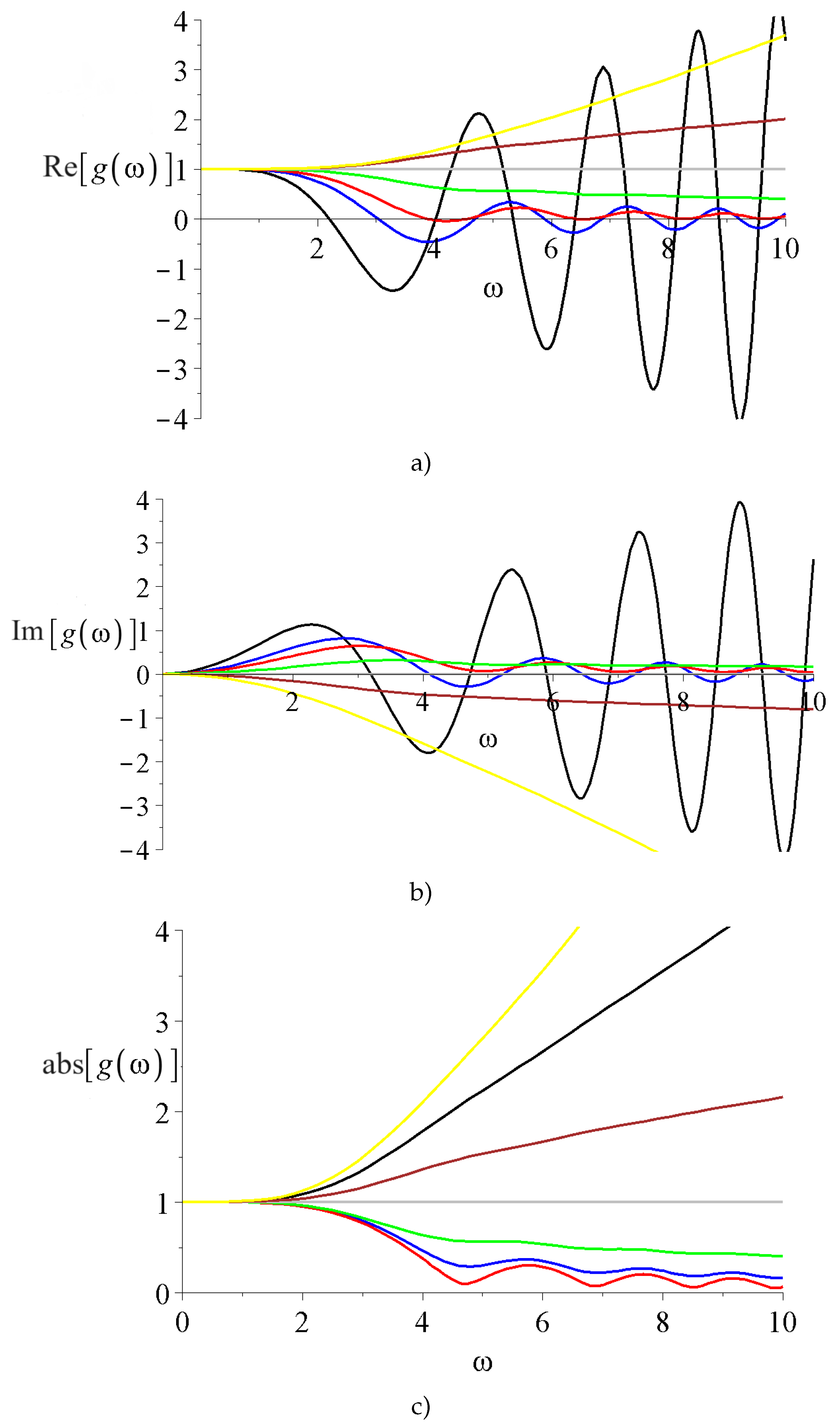
Figure 5.
The and are the real, the complex and the absolute values of the function in Eq. (22) for . The black,blue,red,green, gray, brown and yellow lines are for and , respectively.
Figure 5.
The and are the real, the complex and the absolute values of the function in Eq. (22) for . The black,blue,red,green, gray, brown and yellow lines are for and , respectively.
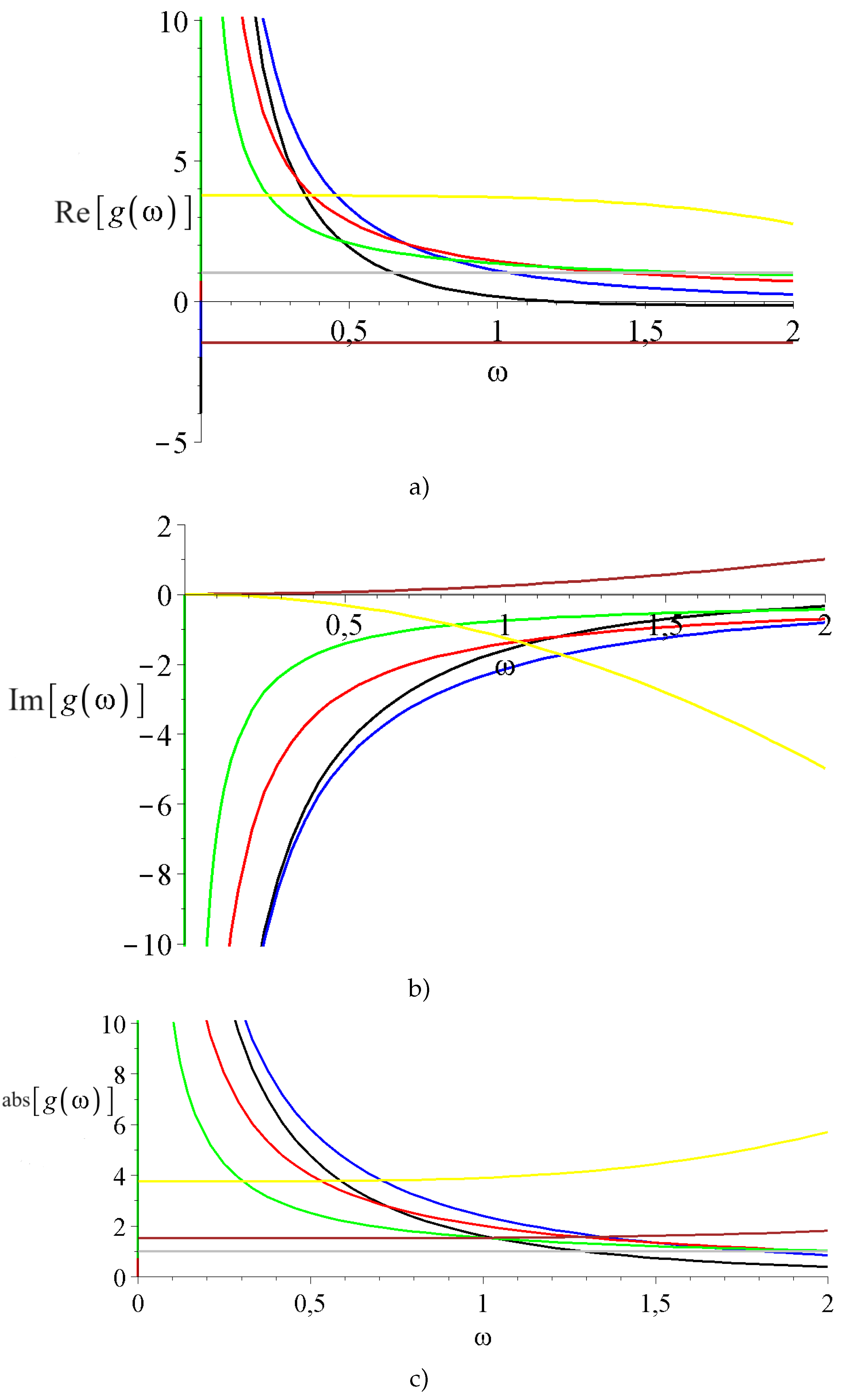
Figure 6.
The possible radial probability particle density in the form of for Eq. (22) with the upper figure shows the Kummer’s M for and the lower one is the Kummer’s U function with , respectively.
Figure 6.
The possible radial probability particle density in the form of for Eq. (22) with the upper figure shows the Kummer’s M for and the lower one is the Kummer’s U function with , respectively.
4. Summary and Outlook
We presented generalized self-similar solutions for the one dimensional Schrödinger equation in Cartesian and spherically symmetric coordinate systems. The solutions can be expressed with the Kummer’s M and Kummer’s U function with complex and quadratic arguments. For some values - which is the new parameter of the solutions - even integrability can be achieved, which mimic a kind of quantum mechanical interperatability. Continuous work is in progress. It seems that additional potential terms can be added to the right hand side of the equations and still analytic results are available. The question of complex angular momenta can be investigated in the near future as well. Additional variable reduction Ansätze (which describes non-classical symmetries) are available too [15] and will be tested to these equations.
Conflicts of Interest
The authors declare no conflict of interest.
References
- Crank, J. The Mathematics of Diffusion; Oxford, Clarendon Press, 1956.
- Ghez, R. Diffusion Phenomena; Dover Publication Inc, 2001.
- Benett, T. Transport by Advection and Diffusion: Momentum, Heat and Mass Transfer,; John Wiley & Sons, 2013.
- Newman, J.; Battaglia, V. The Newman Lectures on Transport Phenomena; Jenny Stanford Publishing, 2021.
- Schiff, L.I. Quantum Mechanics; McGrow-Hill, 1969.
- Sakurai, J.J. Modern Quantum Mechanics (Revised Edition); Addison-Wesley, 1993.
- Messiah, A. Quantum Mechanics; North-Holland Publishing Company, 1961.
- Claude Cohen-Tannoudji, B.D.; Laloë, F. Quantum Mechanics, Volume 1: Basic Concepts, Tools, and Applications; Wiley-VCH, 2019.
- Nagasawa, M. Schrödinger Equation and Diffusion Theory; Springer, 1993.
- Aebi, R. Schrödinger Diffusion Processes; Springer, 2007.
- Barna, I.F.; Rost, J.M. Photoionisation of helium with ultrashort XUV laser pulses. Eur. Phys. J. D 2003, 27, 287–290. [Google Scholar] [CrossRef]
- Barna, I.F.; Pocsai, M.A.; Mátyás, L. Analytic Solutions of the Madelung Equation. Journal of Generalized Lie Theory and Applications 2017, 11, 271. [Google Scholar] [CrossRef]
- Simpao, V.A.; (Editors), H.C.L. Understanding the Sschrödinger Equation Some [Non]Linear Perspectives; Nos Science Publisher, 2020; chapter Chapter 6,Self-Similar and Traveling-Wave Analysis of the Madelung Equations Obtained from the Schrödinger Equation.
- Mátyás, L.; Barna, I.F. General Self-Similar Solutions of Diffusion Equation and Related Constructions. Romanian Journal of Physics 2022, 67, 101–117. doi:https://rjp.nipne.ro/2022_67_1-2/RomJPhys.67.101.pdf.
- Barna, I.F.; Mátyás, L. Advanced Analytic Self-Similar Solutions of Regular and Irregular Diffusion Equations. Mathematics 2022, 10, 3281. [Google Scholar] [CrossRef]
- Mátyás, L.; Barna, I.F. Even and Odd Self-Similar Solutions of the Diffusion Equation for Infinite Horizon. Universe 2023, 9, 264. [Google Scholar] [CrossRef]
- Bluman, G.W.; Cole, J.D. The General Similarity Solution of the Heat Equation. Journal of Mathematics and Mechanics 1969, 18, 1025–1042, https://personal.math.ubc.ca/ bluman/jmm%20article%201969.pdf. [Google Scholar]
- Sedov, L.I. Similarity and Dimensional Methods in Mechanics; CRC Press, 1993.
- Barna, I.F.; Mátyás, L. Analytic self-similar solutions of the Oberbeck–Boussinesq equations. Chaos, Solitons and Fractals 2015, 78, 249–255. [Google Scholar] [CrossRef]
- Barna, I.F.; Bognár, G.; Mátyás, L.; Hriczó, K. Self-similar analysis of the time-dependent compressible and incompressible boundary layers including heat conduction. ournal of Thermal Analysis and Calorimetry 2022, 147, 13625–13632. [Google Scholar] [CrossRef]
- Olver, F.W.J.; Lozier, D.W.; Boisvert, R.F.; Clark, C.W., Eds. NIST Handbook of Mathematical Functions; Cambridge University Press, 2010. doi:https://dlmf.nist.gov/.
- Abramowitz, M.; Stegun, I.E., Eds. Handbook of Mathematical Functions with Formulas, Graphs, and Mathematical Tables; Dover Publisher, 1970.
- Niederer, U. Maximal kinematical invariance group of the free Schrodinger equation. Helv. Phys. Acta 1972, 45, 802–810. [Google Scholar] [CrossRef]
- Shapovalov, V.N.; Bagrov, V.G.; Meshkov, A.G. Izv. Vyssh. Uchebn. Zaved., Fiz.,1971, 8, 45–50. [CrossRef]
- Beckers, J.; Patera, J.; Perroud, M.; Winternitz, P. Subgroups of the Euclidean group and symmetry breaking in nonrelativistic quantum mechanics. J. Math. Phys. 1977, 18, 72–83. [Google Scholar] [CrossRef]
- Berry, M.V.; Balázs, N.L. Nonspreading wave packets. Americal Journal of Physics 1979, 47, 264–267. [Google Scholar] [CrossRef]
- Garraway, B.M.; Suominent, K.A. Wave-packet dynamics: new physics and chemistry in femto-time. Rep, Prog. Phys. 1995, 58, 365–419, https://iopscience.iop.org/article/10.1088/0034-4885/58/4/001/pdf. [Google Scholar]
- Briggs, J.S. Trajectories and the perception of classicalmotion in the free propagation of wave packets. Natural Sciences 2022, 2, 1–18. [Google Scholar] [CrossRef]
- Briggs, J.S.; Rost, J.M. Time dependence in quantum mechanics. European Physical Journal D 2000, 10, 311. [Google Scholar] [CrossRef]
- Gemsheim, S.; Rost, J.M. Emergence of Time from Quantum Interaction with the Environment. Physical Review Letters 2023, 131, 140202. [Google Scholar] [CrossRef] [PubMed]
- Wigner, E. On the Quantum Correction For Thermodynamic Equilibrium. Physical Review 1932, 40, 749. [Google Scholar] [CrossRef]
- Jacobs, K. Quantum Measurement Theory and its Applications; Cambridge University Press, 2014.
- Genovese, M. Research on hidden variable theories: a review of recent progresses. Physics Reports 2005, 413, 319–396. [Google Scholar] [CrossRef]
- Bell, J.S. Speakable and Unspeakable in Quantum Mechanics; Cambridge University Press, 1987.
- Everett, H. Relative State Formulation of Quantum Mechanics. Review of Modern Physics 1957, 29, 454–462. [Google Scholar] [CrossRef]
Disclaimer/Publisher’s Note: The statements, opinions and data contained in all publications are solely those of the individual author(s) and contributor(s) and not of MDPI and/or the editor(s). MDPI and/or the editor(s) disclaim responsibility for any injury to people or property resulting from any ideas, methods, instructions or products referred to in the content. |
© 2023 by the authors. Licensee MDPI, Basel, Switzerland. This article is an open access article distributed under the terms and conditions of the Creative Commons Attribution (CC BY) license (http://creativecommons.org/licenses/by/4.0/).
Copyright: This open access article is published under a Creative Commons CC BY 4.0 license, which permit the free download, distribution, and reuse, provided that the author and preprint are cited in any reuse.